Statistical Modelling
Statistical Modelling
Jump to year
Paper 1, Section I, J
Let . The probability density function of the inverse Gaussian distribution (with the shape parameter equal to 1 ) is given by
Show that this is a one-parameter exponential family. What is its natural parameter? Show that this distribution has mean and variance .
Paper 1, Section II, J
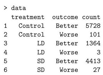
The following data were obtained in a randomised controlled trial for a drug. Due to a manufacturing error, a subset of trial participants received a low dose (LD) instead of a standard dose (SD) of the drug.
(a) Below we analyse the data using Poisson regression:
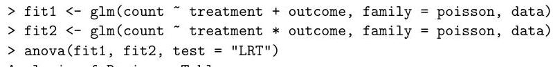
(i) After introducing necessary notation, write down the Poisson models being fitted above.
(ii) Write down the corresponding multinomial models, then state the key theoretical result (the "Poisson trick") that allows you to fit the multinomial models using Poisson regression. [You do not need to prove this theoretical result.]
(iii) Explain why the number of degrees of freedom in the likelihood ratio test is 2 in the analysis of deviance table. What can you conclude about the drug?
(b) Below is the summary table of the second model:
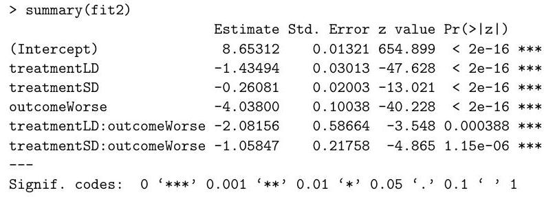
(i) Drug efficacy is defined as one minus the ratio of the probability of worsening in the treated group to the probability of worsening in the control group. By using a more sophisticated method, a published analysis estimated that the drug efficacy is for the LD treatment and for the treatment. Are these numbers similar to what is obtained by Poisson regression? [Hint: , and , where is the base of the natural logarithm.]
(ii) Explain why the information in the summary table is not enough to test the hypothesis that the LD drug and the SD drug have the same efficacy. Then describe how you can test this hypothesis using analysis of deviance in .
Paper 2, Section I, J
Define a generalised linear model for a sample of independent random variables. Define further the concept of the link function. Define the binomial regression model (without the dispersion parameter) with logistic and probit link functions. Which of these is the canonical link function?
Paper 3, Section I, J
Consider the normal linear model , where is a design matrix, is a vector of responses, is the identity matrix, and are unknown parameters.
Derive the maximum likelihood estimator of the pair and . What is the distribution of the estimator of ? Use it to construct a -level confidence interval of . [You may use without proof the fact that the "hat matrix" is a projection matrix.]
Paper 4 , Section I, J
The data frame data contains the daily number of new avian influenza cases in a large poultry farm.

Write down the model being fitted by the code below. Does the model seem to provide a satisfactory fit to the data? Justify your answer.
The owner of the farm estimated that the size of the epidemic was initially doubling every 7 days. Is that estimate supported by the analysis below? [You may need .]


Paper 4, Section II, J
Let be an non-random design matrix and be a -vector of random responses. Suppose , where is an unknown vector and is known.
(a) Let be a constant. Consider the ridge regression problem
Let be the fitted values. Show that , where
(b) Show that
(c) Let , where is independent of . Show that is an unbiased estimator of .
(d) Describe the behaviour (monotonicity and limits) of as a function of when and . What is the minimum value of ?
Paper 1, Section I, J
Consider a generalised linear model with full column rank design matrix , output variables , link function , mean parameters and known dispersion parameters . Denote its variance function by and recall that , where and is the row of .
(a) Define the score function in terms of the log-likelihood function and the Fisher information matrix, and define the update of the Fisher scoring algorithm.
(b) Let be a diagonal matrix with positive entries. Note that is invertible. Show that
[Hint: you may use that
(c) Recall that the score function and the Fisher information matrix have entries
Justify, performing the necessary calculations and using part (b), why the Fisher scoring algorithm is also known as the iterative reweighted least squares algorithm.
Paper 1, Section II, J
We consider a subset of the data on car insurance claims from Hallin and Ingenbleek (1983). For each customer, the dataset includes total payments made per policy-year, the amount of kilometres driven, the bonus from not having made previous claims, and the brand of the car. The amount of kilometres driven is a factor taking values , or 5 , where a car in level has driven a larger number of kilometres than a car in level for any . A statistician from an insurance company fits the following model on .
model1 <- Im(Paymentperpolicyyr as numeric(Kilometres) Brand Bonus)
(i) Why do you think the statistician transformed variable Kilometres from a factor to a numerical variable?
(ii) To check the quality of the model, the statistician applies a function to model1 which returns the following figure:
What does the plot represent? Does it suggest that model1 is a good model? Explain. If not, write down a model which the plot suggests could be better.
(iii) The statistician fits the model suggested by the graph and calls it model2. Consider the following abbreviated output:
Coefficients:
Brand2
Brand9
Bonus

Signif. codes: 0 '' '' '' '.' ' 1
Residual standard error: on 284 degrees of freedom ..
Using the output, write down a prediction interval for the ratio between the total payments per policy year for two cars of the same brand and with the same value of Bonus, one of which has a Kilometres value one higher than the other. You may express your answer as a function of quantiles of a common distribution, which you should specify.
(iv) Write down a generalised linear model for Paymentperpolicyyr which may be a better model than model1 and give two reasons. You must specify the link function.
Paper 2, Section I, J
The data frame WCG contains data from a study started in 1960 about heart disease. The study used 3154 adult men, all free of heart disease at the start, and eight and a half years later it recorded into variable chd whether they suffered from heart disease (1 if the respective man did and 0 otherwise) along with their height and average number of cigarettes smoked per day. Consider the code below and its abbreviated output.

(a) Write down the model fitted by the code above.
(b) Interpret the effect on heart disease of a man smoking an average of two packs of cigarettes per day if each pack contains 20 cigarettes.
(c) Give an alternative latent logistic-variable representation of the model. [Hint: if is the cumulative distribution function of a logistic random variable, its inverse function is the logit function.]
Paper 3, Section I, J
Suppose we have data , where the are independent conditional on the design matrix whose rows are the . Suppose that given , the true probability density function of is , so that the data is generated from an element of a model for some and .
(a) Define the log-likelihood function for , the maximum likelihood estimator of and Akaike's Information Criterion (AIC) for .
From now on let be the normal linear model, i.e. , where has full column rank and .
(b) Let denote the maximum likelihood estimator of . Show that the AIC of is
(c) Let be a chi-squared distribution on degrees of freedom. Using any results from the course, show that the distribution of the AIC of is
Hint: , where is the maximum likelihood estimator of and is the projection matrix onto the column space of .]
Paper 4, Section I, J
Suppose you have a data frame with variables response, covar1, and covar2. You run the following commands on .

...
(a) Consider the following three scenarios:
(i) All the output you have is the abbreviated output of summary (model) above.
(ii) You have the abbreviated output of summary (model) above together with
Residual standard error: on 47 degrees of freedom
Multiple R-squared: , Adjusted R-squared:
F-statistic: on 2 and 47 DF, p-value: <
(iii) You have the abbreviated output of summary (model) above together with
Residual standard error: on 47 degrees of freedom
Multiple R-squared: , Adjusted R-squared:
F-statistic: on 2 and 47 DF, p-value:
What conclusion can you draw about which variables explain the response in each of the three scenarios? Explain.
(b) Assume now that you have the abbreviated output of summary (model) above together with
anova(lm(response response , model
What are the values of the entries with a question mark? [You may express your answers as arithmetic expressions if necessary].
Paper 4, Section II, J
(a) Define a generalised linear model with design matrix , output variables and parameters and . Derive the moment generating function of , i.e. give an expression for , wherever it is well-defined.
Assume from now on that the GLM satisfies the usual regularity assumptions, has full column rank, and is known and satisfies .
(b) Let be the output variables of a GLM from the same family as that of part (a) and parameters and . Suppose the output variables may be split into blocks of size with constant parameters. To be precise, for each block , if then
with and defined as in part a . Let , where .
(i) Show that is equal to in distribution. [Hint: you may use without proof that moment generating functions uniquely determine distributions from exponential dispersion families.]
(ii) For any , let , where . Show that the model function of satisfies
for some functions , and conclude that is a sufficient statistic for from .
(iii) For the model and data from part (a), let be the maximum likelihood estimator for and let be the deviance at . Using (i) and (ii), show that
where means equality in distribution and and are nested subspaces of which you should specify. Argue that and , and, assuming the usual regularity assumptions, conclude that
stating the name of the result from class that you use.
Paper 1, Section I, J
The Gamma distribution with shape parameter and scale parameter has probability density function
Give the definition of an exponential dispersion family and show that the set of Gamma distributions forms one such family. Find the cumulant generating function and derive the mean and variance of the Gamma distribution as a function of and .
Paper 1, Section II, J
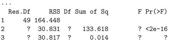
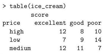
The ice_cream data frame contains the result of a blind tasting of 90 ice creams, each of which is rated as poor, good, or excellent. It also contains the price of each ice cream classified into three categories. Consider the code below and its output.
(a) Write down the generalised linear model fitted by the code above.
(b) Prove that the fitted values resulting from the maximum likelihood estimator of the coefficients in this model are identical to those resulting from the maximum likelihood estimator when fitting a Multinomial model which assumes the number of ice creams at each price level is fixed.
(c) Using the output above, perform a goodness-of-fit test at the level, specifying the null hypothesis, the test statistic, its asymptotic null distribution, any assumptions of the test and the decision from your test. (d) If we believe that better ice creams are more expensive, what could be a more powerful test against the model fitted above and why?
Paper 2, Section I, J
The cycling data frame contains the results of a study on the effects of cycling to work among 1,000 participants with asthma, a respiratory illness. Half of the participants, chosen uniformly at random, received a monetary incentive to cycle to work, and the other half did not. The variables in the data frame are:
miles: the average number of miles cycled per week
episodes: the number of asthma episodes experienced during the study
incentive: whether or not a monetary incentive to cycle was given
history: the number of asthma episodes in the year preceding the study
Consider the code below and its abbreviated output.
(episodes miles history, data=cycling)
Coefficients:
Estimate Std. Error value
(Intercept)
miles
history
episodes incentive history, data=cycling)
summary (lm.2)
Coefficients:
Estimate Std. Error value
(Intercept)
incentiveYes
history
miles incentive history, data=cycling)
Coefficients :
Estimate Std. Error t value
(Intercept)
incentiveYes
history
(a) For each of the fitted models, briefly explain what can be inferred about participants with similar histories.
(b) Based on this analysis and the experimental design, is it advisable for a participant with asthma to cycle to work more often? Explain.
Paper 3, Section I, J
(a) For a given model with likelihood , define the Fisher information matrix in terms of the Hessian of the log-likelihood.
Consider a generalised linear model with design matrix , output variables , a bijective link function, mean parameters and dispersion parameters . Assume is known.
(b) State the form of the log-likelihood.
(c) For the canonical link, show that when the parameter is known, the Fisher information matrix is equal to
for a diagonal matrix depending on the means . Identify .
Paper 4, Section I, J
In a normal linear model with design matrix , output variables and parameters and , define a -level prediction interval for a new observation with input variables . Derive an explicit formula for the interval, proving that it satisfies the properties required by the definition. [You may assume that the maximum likelihood estimator is independent of , which has a distribution.]
Paper 4, Section II, J
A sociologist collects a dataset on friendships among Cambridge graduates. Let if persons and are friends 3 years after graduation, and otherwise. Let be a categorical variable for person 's college, taking values in the set . Consider logistic regression models,
with parameters either
; or,
; or,
, where if and 0 otherwise.
(a) Write the likelihood of the models.
(b) Show that the three models are nested and specify the order. Suggest a statistic to compare models 1 and 3, give its definition and specify its asymptotic distribution under the null hypothesis, citing any necessary theorems.
(c) Suppose persons and are in the same college consider the number of friendships, and , that each of them has with people in college ( and fixed). In each of the models above, compare the distribution of these two random variables. Explain why this might lead to a poor quality of fit.
(d) Find a minimal sufficient statistic for model 3. [You may use the following characterisation of a minimal sufficient statistic: let be the likelihood in this model, where and suppose is a statistic such that is constant in if and only if ; then, is a minimal sufficient statistic for .]
Paper 1, Section I, J
The data frame Ambulance contains data on the number of ambulance requests from a Cambridgeshire hospital on different days. In addition to the number of ambulance requests on each day, the dataset records whether each day fell in the winter season, on a weekend, or on a bank holiday, as well as the pollution level on each day.
A health researcher fitted two models to the dataset above using . Consider the following code and its output.


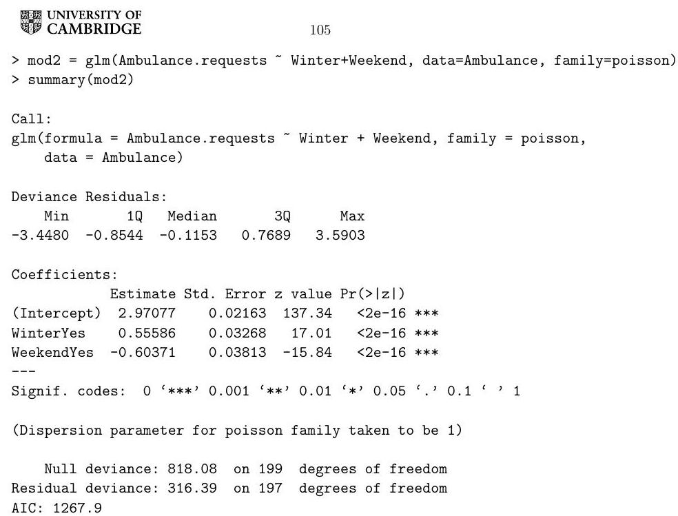
Define the two models fitted by this code and perform a hypothesis test with level in which one of the models is the null hypothesis and the other is the alternative. State the theorem used in this hypothesis test. You may use the information generated by the following commands.
Paper 1, Section II, J
A clinical study follows a number of patients with an illness. Let be the length of time that patient lives and a vector of predictors, for . We shall assume that are independent. Let and be the probability density function and cumulative distribution function, respectively, of . The hazard function is defined as
We shall assume that , where is a vector of coefficients and is some fixed hazard function.
(a) Prove that .
(b) Using the equation in part (a), write the log-likelihood function for in terms of and only.
(c) Show that the maximum likelihood estimate of can be obtained through a surrogate Poisson generalised linear model with an offset.
Paper 2, Section I,
Consider a linear model with , where the design matrix is by . Provide an expression for the -statistic used to test the hypothesis for . Show that it is a monotone function of a log-likelihood ratio statistic.
Paper 3, Section I, J
The data frame Cases. of .flu contains a list of cases of flu recorded in 3 London hospitals during each month of 2017 . Consider the following code and its output.
table (Cases. of.flu)
Month Hospital
May
November
October
September
Cases. of.flu.table = as.data.frame (table (Cases. of .flu))
head (Cases. of .flu.table)
Month Hospital Freq
1 April A 10
2 August A 9
3 December A 24
4 February A 49
5 January A 45
6 July A 5
glm (Freq ., data=Cases. of .flu.table, family=poisson)
[1]
levels (Cases. of.flu$Month)

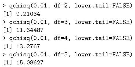
Describe a test for the null hypothesis of independence between the variables Month and Hospital using the deviance statistic. State the assumptions of the test.
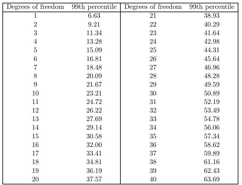
Perform the test at the level for each of the two different models shown above. You may use the table below showing 99 th percentiles of the distribution with a range of degrees of freedom . How would you explain the discrepancy between their conclusions?
Paper 4, Section I, J
A scientist is studying the effects of a drug on the weight of mice. Forty mice are divided into two groups, control and treatment. The mice in the treatment group are given the drug, and those in the control group are given water instead. The mice are kept in 8 different cages. The weight of each mouse is monitored for 10 days, and the results of the experiment are recorded in the data frame Weight.data. Consider the following code and its output.
head (Weight.data)
Time Group Cage Mouse Weight
11 Control 1 1
Control 1 1
Control
44 Control
Control 1 1
Control
(Weight Time*Group Cage, data=Weight. data)
Call:
(formula Weight Time Group Cage, data Weight. data)
Residuals:
Min Median Max
Coefficients:
Estimate Std. Error t value
GroupTreatment
Cage2
Time: GroupTreatment
Signif. codes: 0 '' '' '' '., ', 1
Residual standard error: on 391 degrees of freedom
Multiple R-squared: , Adjusted R-squared:
F-statistic: on 8 and 391 DF, p-value:
Which parameters describe the rate of weight loss with time in each group? According to the output, is there a statistically significant weight loss with time in the control group?
Three diagnostic plots were generated using the following code.

Weight.data$Time[mouse1]

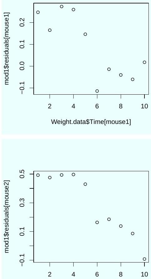
Weight.data$Time[mouse2]
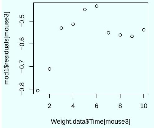
Based on these plots, should you trust the significance tests shown in the output of the command summary (mod1)? Explain.
Paper 4, Section II, J
Bridge is a card game played by 2 teams of 2 players each. A bridge club records the outcomes of many games between teams formed by its members. The outcomes are modelled by
where is a parameter representing the skill of player , and is a parameter representing how well-matched the team formed by and is.
(a) Would it make sense to include an intercept in this logistic regression model? Explain your answer.
(b) Suppose that players 1 and 2 always play together as a team. Is there a unique maximum likelihood estimate for the parameters and ? Explain your answer.
(c) Under the model defined above, derive the asymptotic distribution (including the values of all relevant parameters) for the maximum likelihood estimate of the probability that team wins a game against team . You can state it as a function of the true vector of parameters , and the Fisher information matrix with games. You may assume that as , and that has a unique maximum likelihood estimate for large enough.
Paper 1, Section I, J
The dataset ChickWeights records the weight of a group of chickens fed four different diets at a range of time points. We perform the following regressions in .
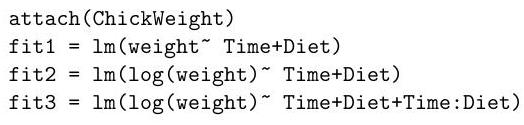
(i) Which hypothesis test does the following command perform? State the degrees of freedom, and the conclusion of the test.
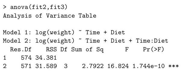
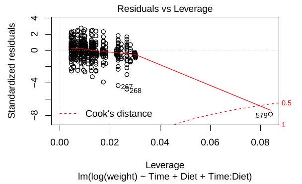
(ii) Define a diagnostic plot that might suggest the logarithmic transformation of the response in fit2.
(iii) Define the dashed line in the following plot, generated with the command plot(fit3). What does it tell us about the data point 579 ?
Paper 1, Section II, J
The Cambridge Lawn Tennis Club organises a tournament in which every match consists of 11 games, all of which are played. The player who wins 6 or more games is declared the winner.
For players and , let be the total number of games they play against each other, and let be the number of these games won by player . Let and be the corresponding number of matches.
A statistician analysed the tournament data using a Binomial Generalised Linear Model (GLM) with outcome . The probability that wins a game against is modelled by
with an appropriate corner point constraint. You are asked to re-analyse the data, but the game-level results have been lost and you only know which player won each match.
We define a new GLM for the outcomes with and , where the are defined in . That is, is the log-odds that wins a game against , not a match.
Derive the form of the new link function . [You may express your answer in terms of a cumulative distribution function.]
Paper 2, Section I, J
A statistician is interested in the power of a -test with level in linear regression; that is, the probability of rejecting the null hypothesis with this test under an alternative with .
(a) State the distribution of the least-squares estimator , and hence state the form of the -test statistic used.
(b) Prove that the power does not depend on the other coefficients for .
Paper 3, Section I, J
For Fisher's method of Iteratively Reweighted Least-Squares and Newton-Raphson optimisation of the log-likelihood, the vector of parameters is updated using an iteration
for a specific function . How is defined in each method?
Prove that they are identical in a Generalised Linear Model with the canonical link function.
Paper 4, Section I, J
A Cambridge scientist is testing approaches to slow the spread of a species of moth in certain trees. Two groups of 30 trees were treated with different organic pesticides, and a third group of 30 trees was kept under control conditions. At the end of the summer the trees are classified according to the level of leaf damage, obtaining the following contingency table.

Which of the following Generalised Linear Model fitting commands is appropriate for these data? Why? Describe the model being fit.
Paper 4, Section II, J
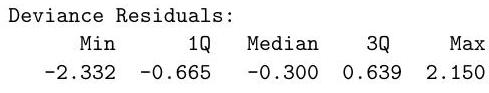
The dataset diesel records the number of diesel cars which go through a block of Hills Road in 6 disjoint periods of 30 minutes, between 8AM and 11AM. The measurements are repeated each day for 10 days. Answer the following questions based on the code below, which is shown with partial output.
(a) Can we reject the model fit. 1 at a level? Justify your answer.
(b) What is the difference between the deviance of the models fit. 2 and fit.3?
(c) Which of fit. 2 and fit. 3 would you use to perform variable selection by backward stepwise selection? Why?
(d) How does the final plot differ from what you expect under the model in fit.2? Provide a possible explanation and suggest a better model.
head (diesel)
period num.cars day
fit. glm(num.cars period, data=diesel, family=poisson)
summary (fit.1)
Deviance Residuals:
Min 1Q Median 3Q Max
Coefficients:
Estimate Std. Error value
(Intercept)
period
Signif. codes: 0 ? ? ? ? ?.? ? ? 1
(Dispersion parameter for poisson family taken to be 1)
Null deviance: on 59 degrees of freedom
Residual deviance: on 58 degrees of freedom
AIC:
diesel$period.factor = factor(diesel$period)
fit. glm (num.cars period.factor, data=diesel, family=poisson)
(fit.2)
Coefficients:
Estimate Std. Error z value

Part II, List of Questions
[TURN OVER
Paper 1, Section I, K
The body mass index (BMI) of your closest friend is a good predictor of your own BMI. A scientist applies polynomial regression to understand the relationship between these two variables among 200 students in a sixth form college. The commands
fit. poly friendBMI , 2, raw=T
fit. poly friendBMI, 3, raw
fit the models and , respectively, with in each case.
Setting the parameters raw to FALSE:
fit. poly friendBMI , 2, raw=F )
fit. poly friendBMI, 3, raw
fits the models and , with . The function is a polynomial of degree . Furthermore, the design matrix output by the function poly with raw=F satisfies:
poly friendBMI, 3, raw poly , raw
How does the variance of differ in the models and ? What about the variance of the fitted values ? Finally, consider the output of the commands
(fit.1,fit.2)
anova(fit.3,fit.4)
Define the test statistic computed by this function and specify its distribution. Which command yields a higher statistic?
Paper 1, Section II, K
(a) Let be an -vector of responses from the linear model , with . The internally studentized residual is defined by
where is the least squares estimate, is the leverage of sample , and
Prove that the joint distribution of is the same in the following two models: (i) , and (ii) , with (in this model, are identically -distributed). [Hint: A random vector is spherically symmetric if for any orthogonal matrix . If is spherically symmetric and a.s. nonzero, then is a uniform point on the sphere; in addition, any orthogonal projection of is also spherically symmetric. A standard normal vector is spherically symmetric.]
(b) A social scientist regresses the income of 120 Cambridge graduates onto 20 answers from a questionnaire given to the participants in their first year. She notices one questionnaire with very unusual answers, which she suspects was due to miscoding. The sample has a leverage of . To check whether this sample is an outlier, she computes its externally studentized residual,
where is estimated from a fit of all samples except the one in question, . Is this a high leverage point? Can she conclude this sample is an outlier at a significance level of ?
(c) After examining the following plot of residuals against the response, the investigator calculates the externally studentized residual of the participant denoted by the black dot, which is . Can she conclude this sample is an outlier with a significance level of ?
Part II, List of Questions
Paper 2, Section I, K
Define an exponential dispersion family. Prove that the range of the natural parameter, , is an open interval. Derive the mean and variance as a function of the log normalizing constant.
[Hint: Use the convexity of , i.e. for all
Paper 3, Section I, K
The command
rainfall month+elnino+month:elnino)
performs a Box-Cox transform of the response at several values of the parameter , and produces the following plot:
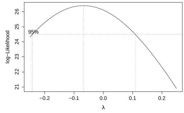
We fit two linear models and obtain the Q-Q plots for each fit, which are shown below in no particular order:
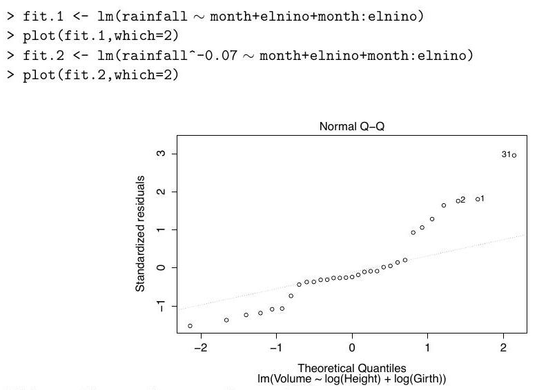
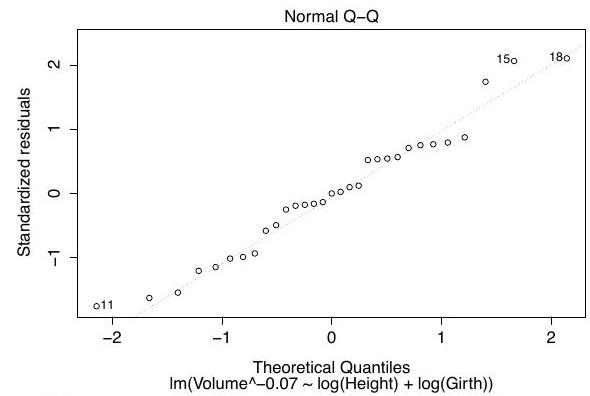
Define the variable on the -axis in the output of boxcox, and match each Q-Q plot to one of the models.
After choosing the model fit.2, the researcher calculates Cook's distance for the th sample, which has high leverage, and compares it to the upper -point of an distribution, because the design matrix is of size . Provide an interpretation of this comparison in terms of confidence sets for . Is this confidence statement exact?
Paper 4, Section I, K
(a) Let where for are independent and identically distributed. Let for , and suppose that these variables follow a binary regression model with the complementary log-log link function . What is the probability density function of ?
(b) The Newton-Raphson algorithm can be applied to compute the MLE, , in certain GLMs. Starting from , we let be the maximizer of the quadratic approximation of the log-likelihood around :
where and are the gradient and Hessian of the log-likelihood. What is the difference between this algorithm and Iterative Weighted Least Squares? Why might the latter be preferable?
Paper 4, Section II, K
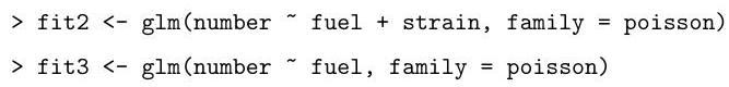
For 31 days after the outbreak of the 2014 Ebola epidemic, the World Health Organization recorded the number of new cases per day in 60 hospitals in West Africa. Researchers are interested in modelling , the number of new Ebola cases in hospital on day , as a function of several covariates:
lab: a Boolean factor for whether the hospital has laboratory facilities,
casesBefore: number of cases at the hospital on the previous day,
urban: a Boolean factor indicating an urban area,
country: a factor with three categories, Guinea, Liberia, and Sierra Leone,
numDoctors: number of doctors at the hospital,
tradBurials: a Boolean factor indicating whether traditional burials are common in the region.
Consider the output of the following code (with some lines omitted):
fit. 1 <- glm(newCases lab+casesBefore+urban+country+numDoctors+tradBurials,
- data=ebola, family=poisson)
summary (fit.1)
Coefficients:
Estimate Std. Error z value
casesBefore
countryLiberia
countrySierra Leone
numDoctors
tradBurialstrUE
Signif. codes:
(a) Would you conclude based on the -tests that an urban setting does not affect the rate of infection?
(b) Explain how you would predict the total number of new cases that the researchers will record in Sierra Leone on day 32 .
We fit a new model which includes an interaction term, and compute a test statistic using the code:
fit. glm (newCases casesBefore+country+country:casesBefore+numDoctors,
- data=ebola, family=poisson)
fit. 2 deviance - fit.1$deviance
[1]
(c) What is the distribution of the statistic computed in the last line?
(d) Under what conditions is the deviance of each model approximately chi-squared?
Paper 1, Section I, J
The outputs of a particular process are positive and are believed to be related to -vectors of covariates according to the following model
In this model are i.i.d. random variables where is known. It is not possible to measure the output directly, but we can detect whether the output is greater than or less than or equal to a certain known value . If
show that a probit regression model can be used for the data .
How can we recover and from the parameters of the probit regression model?
Paper 1, Section II, J
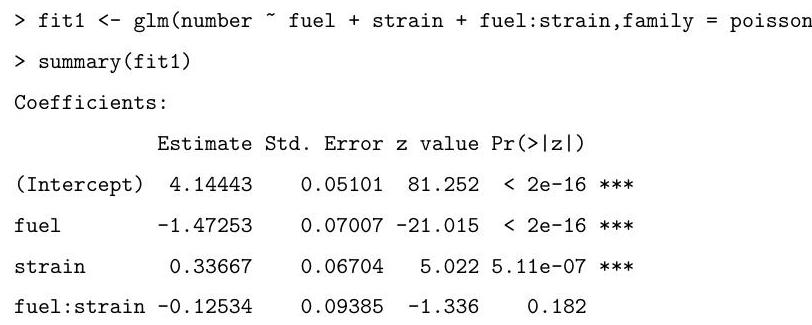
An experiment is conducted where scientists count the numbers of each of three different strains of fleas that are reproducing in a controlled environment. Varying concentrations of a particular toxin that impairs reproduction are administered to the fleas. The results of the experiment are stored in a data frame in , whose first few rows are given below.
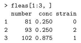
The full dataset has 80 rows. The first column provides the number of fleas, the second provides the concentration of the toxin and the third specifies the strain of the flea as factors 0,1 or 2 . Strain 0 is the common flea and strains 1 and 2 have been genetically modified in a way thought to increase their ability to reproduce in the presence of the toxin.
Explain and interpret the commands and (abbreviated) output below. In particular, you should describe the model being fitted, briefly explain how the standard errors are calculated, and comment on the hypothesis tests being described in the summary.

Explain and motivate the following code in the light of the output above. Briefly explain the differences between the models fitted below, and the model corresponding to it
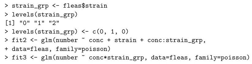
Denote by the three models being fitted in sequence above. Explain the hypothesis tests comparing the models to each other that can be performed using the output from the following code.
fit1$dev, fit2$dev, fit3$dev)
[1]
[1]
Use these numbers to comment on the most appropriate model for the data.
Paper 2, Section I, J
Let be independent Poisson random variables with means , where for some known constants and an unknown parameter . Find the log-likelihood for .
By first computing the first and second derivatives of the log-likelihood for , describe the algorithm you would use to find the maximum likelihood estimator . Hint: Recall that if then
for .]
Paper 3, Section I, J
Data are available on the number of counts (atomic disintegration events that take place within a radiation source) recorded with a Geiger counter at a nuclear plant. The counts were registered at each second over a 30 second period for a short-lived, man-made radioactive compound. The first few rows of the dataset are displayed below.

Describe the model being fitted with the following command.
fit Counts Time, data=geiger)
Below is a plot against time of the residuals from the model fitted above.

Referring to the plot, suggest how the model could be improved, and write out the code for fitting this new model. Briefly describe how one could test in whether the new model is to be preferred over the old model.
Paper 4, Section I, J
Data on 173 nesting female horseshoe crabs record for each crab its colour as one of 4 factors (simply labelled ), its width (in ) and the presence of male crabs nearby (a 1 indicating presence). The data are collected into the data frame crabs and the first few lines are displayed below.

Describe the model being fitted by the command below.
fit1 <- glm(males colour + width, family = binomial, data=crabs)
The following (abbreviated) output is obtained from the summary command.

Write out the calculation for an approximate confidence interval for the coefficient for width. Describe the calculation you would perform to obtain an estimate of the probability that a female crab of colour 3 and with a width of has males nearby. [You need not actually compute the end points of the confidence interval or the estimate of the probability above, but merely show the calculations that would need to be performed in order to arrive at them.]
Paper 4, Section II, J
Consider the normal linear model where the -vector of responses satisfies with . Here is an matrix of predictors with full column rank where and is an unknown vector of regression coefficients. For , denote the th column of by , and let be with its th column removed. Suppose where is an -vector of 1 's. Denote the maximum likelihood estimate of by . Write down the formula for involving , the orthogonal projection onto the column space of .
Consider with . By thinking about the orthogonal projection of onto , show that
[You may use standard facts about orthogonal projections including the fact that if and are subspaces of with a subspace of and and denote orthogonal projections onto and respectively, then for all .]
By considering the fitted values , explain why if, for any , a constant is added to each entry in the th column of , then will remain unchanged. Let . Why is (*) also true when all instances of and are replaced by and respectively?
The marks from mid-year statistics and mathematics tests and an end-of-year statistics exam are recorded for 100 secondary school students. The first few lines of the data are given below.

The following abbreviated output is obtained:

What are the hypothesis tests corresponding to the final column of the coefficients table? What is the hypothesis test corresponding to the final line of the output? Interpret the results when testing at the level.
How does the following sample correlation matrix for the data help to explain the relative sizes of some of the -values?

Paper 1, Section , K
Write down the model being fitted by the following command, where and is an matrix with real-valued entries.
fit poisson)
Write down the log-likelihood for the model. Explain why the command
predict (fit, type "response"
gives the answer 0, by arguing based on the log-likelihood you have written down. [Hint: Recall that if then
for .]
Paper 1, Section II,
Consider the normal linear model where the -vector of responses satisfies with . Here is an matrix of predictors with full column rank where , and is an unknown vector of regression coefficients. Let be the matrix formed from the first columns of , and partition as where and . Denote the orthogonal projections onto the column spaces of and by and respectively.
It is desired to test the null hypothesis against the alternative hypothesis . Recall that the -test for testing against rejects for large values of
Show that , and hence prove that the numerator and denominator of are independent under either hypothesis.
Show that
where .
[In this question you may use the following facts without proof: is an orthogonal projection with rank ; any orthogonal projection matrix satisfies , where and if then when
Paper 2, Section I, K
Define the concept of an exponential dispersion family. Show that the family of scaled binomial distributions , with and , is of exponential dispersion family form.
Deduce the mean of the scaled binomial distribution from the exponential dispersion family form.
What is the canonical link function in this case?
Paper 3, Section I,
In an experiment to study factors affecting the production of the plastic polyvinyl chloride , three experimenters each used eight devices to produce the PVC and measured the sizes of the particles produced. For each of the 24 combinations of device and experimenter, two size measurements were obtained.
The experimenters and devices used for each of the 48 measurements are stored in as factors in the objects experimenter and device respectively, with the measurements themselves stored in the vector psize. The following analysis was performed in .
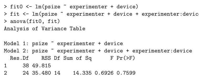
Let and denote the design matrices obtained by model.matrix(fit) and model.matrix (fit0) respectively, and let denote the response psize. Let and denote orthogonal projections onto the column spaces of and respectively.
For each of the following quantities, write down their numerical values if they appear in the analysis of variance table above; otherwise write 'unknown'.
Out of the two models that have been fitted, which appears to be the more appropriate for the data according to the analysis performed, and why?
Paper 4, Section I,
Consider the normal linear model where the -vector of responses satisfies with and is an design matrix with full column rank. Write down a -level confidence set for .
Define the Cook's distance for the observation where is the th row of , and give its interpretation in terms of confidence sets for .
In the model above with and , you observe that one observation has Cook's distance 3.1. Would you be concerned about the influence of this observation? Justify your answer.
[Hint: You may find some of the following facts useful:
If , then .
If , then .
If , then
Paper 4, Section II, K
In a study on infant respiratory disease, data are collected on a sample of 2074 infants. The information collected includes whether or not each infant developed a respiratory disease in the first year of their life; the gender of each infant; and details on how they were fed as one of three categories (breast-fed, bottle-fed and supplement). The data are tabulated in as follows:
Write down the model being fit by the commands on the following page:

The following (slightly abbreviated) output from is obtained.
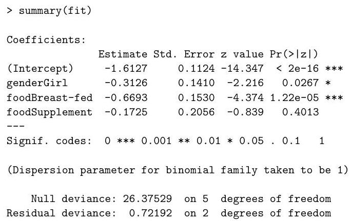
Briefly explain the justification for the standard errors presented in the output above.
Explain the relevance of the output of the following code to the data being studied, justifying your answer:
[1]
[Hint: It may help to recall that if then
Let be the deviance of the model fitted by the following command.
fit glm (disease/total gender + food + gender:food,
family = binomial, weights = total
What is the numerical value of ? Which of the two models that have been fitted should you prefer, and why?
Paper 1, Section I, J
Variables are independent, with having a density governed by an unknown parameter . Define the deviance for a model that imposes relationships between the .
From this point on, suppose . Write down the log-likelihood of data as a function of .
Let be the maximum likelihood estimate of under model . Show that the deviance for this model is given by
Now suppose that, under , where are known -dimensional explanatory variables and is an unknown -dimensional parameter. Show that satisfies , where and is the matrix with rows , and express this as an equation for the maximum likelihood estimate of . [You are not required to solve this equation.]
Paper 1, Section II, J
A cricket ball manufacturing company conducts the following experiment. Every day, a bowling machine is set to one of three levels, "Medium", "Fast" or "Spin", and then bowls 100 balls towards the stumps. The number of times the ball hits the stumps and the average wind speed (in kilometres per hour) during the experiment are recorded, yielding the following data (abbreviated):
Write down a reasonable model for , where is the number of times the ball hits the stumps on the day. Explain briefly why we might want to include interactions between the variables. Write code to fit your model.
The company's statistician fitted her own generalized linear model using , and obtained the following summary (abbreviated):
Why are LevelMedium and Wind: LevelMedium not listed?
Suppose that, on another day, the bowling machine is set to "Spin", and the wind speed is 5 kilometres per hour. What linear function of the parameters should the statistician use in constructing a predictor of the number of times the ball hits the stumps that day?
Based on the above output, how might you improve the model? How could you fit your new model in ?
Paper 2, Section I, J
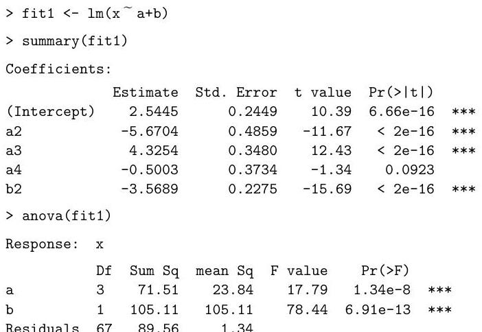
Consider a linear model , where and are with , is , and is of full . Let and be sub-vectors of . What is meant by orthogonality between and ?
Now suppose
where are independent random variables, are real-valued known explanatory variables, and is a cubic polynomial chosen so that is orthogonal to and is orthogonal to .
Let . Describe the matrix such that . Show that is block diagonal. Assuming further that this matrix is non-singular, show that the least-squares estimators of and are, respectively,
Paper 3, Section I, J
Consider the linear model where , and , with independent random variables. The matrix is known and is of full rank . Give expressions for the maximum likelihood estimators and of and respectively, and state their joint distribution. Show that is unbiased whereas is biased.
Suppose that a new variable is to be observed, satisfying the relationship
where is known, and independently of . We propose to predict by . Identify the distribution of
where
Paper 4, Section I, J
The output of a process depends on the levels of two adjustable variables: , a factor with four levels, and , a factor with two levels. For each combination of a level of and a level of , nine independent values of are observed.
Explain and interpret the commands and (abbreviated) output below. In particular, describe the model being fitted, and describe and comment on the hypothesis tests performed under the summary and anova commands.
Paper 4, Section II, J
Let be a probability density function, with cumulant generating function . Define what it means for a random variable to have a model function of exponential dispersion family form, generated by .
A random variable is said to have an inverse Gaussian distribution, with parameters and (both positive), if its density function is
Show that the family of all inverse Gaussian distributions for is of exponential dispersion family form. Deduce directly the corresponding expressions for and in terms of and . What are the corresponding canonical link function and variance function?
Consider a generalized linear model, , for independent variables , whose random component is defined by the inverse Gaussian distribution with link function thus , where is the vector of unknown regression coefficients and is the vector of known values of the explanatory variables for the observation. The vectors are linearly independent. Assuming that the dispersion parameter is known, obtain expressions for the score function and Fisher information matrix for . Explain how these can be used to compute the maximum likelihood estimate of .
Paper 1, Section I, K
Let be independent with , and
where is a vector of regressors and is a vector of parameters. Write down the likelihood of the data as a function of . Find the unrestricted maximum likelihood estimator of , and the form of the maximum likelihood estimator under the logistic model (1).
Show that the deviance for a comparison of the full (saturated) model to the generalised linear model with canonical link (1) using the maximum likelihood estimator can be simplified to
Finally, obtain an expression for the deviance residual in this generalised linear model.
Paper 1, Section II, K
The treatment for a patient diagnosed with cancer of the prostate depends on whether the cancer has spread to the surrounding lymph nodes. It is common to operate on the patient to obtain samples from the nodes which can then be analysed under a microscope. However it would be preferable if an accurate assessment of nodal involvement could be made without surgery. For a sample of 53 prostate cancer patients, a number of possible predictor variables were measured before surgery. The patients then had surgery to determine nodal involvement. We want to see if nodal involvement can be accurately predicted from the available variables and determine which ones are most important. The variables take the values 0 or 1 .
An indicator no yes of nodal involvement.
aged The patient's age, split into less than and 60 or over .
stage A measurement of the size and position of the tumour observed by palpation with the fingers. A serious case is coded as 1 and a less serious case as 0 .
grade Another indicator of the seriousness of the cancer which is determined by a pathology reading of a biopsy taken by needle before surgery. A value of 1 indicates a more serious case of cancer.
xray Another measure of the seriousness of the cancer taken from an X-ray reading. A value of 1 indicates a more serious case of cancer.
acid The level of acid phosphatase in the blood serum where high and low.
A binomial generalised linear model with a logit link was fitted to the data to predict nodal involvement and the following output obtained:
Part II, 2012 List of Questions
[TURN OVER (a) Give an interpretation of the coefficient of xray.
(b) Give the numerical value of the sum of the squared deviance residuals.
(c) Suppose that the predictors, stage, grade and xray are positively correlated. Describe the effect that this correlation is likely to have on our ability to determine the strength of these predictors in explaining the response.
(d) The probability of observing a value of under a Chi-squared distribution with 52 degrees of freedom is . What does this information tell us about the null model for this data? Justify your answer.
(e) What is the lowest predicted probability of the nodal involvement for any future patient?
(f) The first plot in Figure 1 shows the (Pearson) residuals and the fitted values. Explain why the points lie on two curves.
(g) The second plot in Figure 1 shows the value of where indicates that patient was dropped in computing the fit. The values for each predictor, including the intercept, are shown. Could a single case change our opinion of which predictors are important in predicting the response?

Figure 1: The plot on the left shows the Pearson residuals and the fitted values. The plot on the right shows the changes in the regression coefficients when a single point is omitted for each predictor.
Paper 2, Section I, K
The purpose of the following study is to investigate differences among certain treatments on the lifespan of male fruit flies, after allowing for the effect of the variable 'thorax length' (thorax) which is known to be positively correlated with lifespan. Data was collected on the following variables:
longevity lifespan in days
thorax (body) length in
treat a five level factor representing the treatment groups. The levels were labelled as follows: "00", "10", "80", "11", "81".
No interactions were found between thorax length and the treatment factor. A linear model with thorax as the covariate, treat as a factor (having the above 5 levels) and longevity as the response was fitted and the following output was obtained. There were 25 males in each of the five groups, which were treated identically in the provision of fresh food.
Coefficients :
Residual standard error: on 119 degrees of freedom
Multiple R-Squared: , Adjusted R-squared:
F-statistics: on 5 and 119 degrees of freedom, p-value: 0
(a) Assuming the same treatment, how much longer would you expect a fly with a thorax length greater than another to live?
(b) What is the predicted difference in longevity between a male fly receiving treatment treat 10 and treat81 assuming they have the same thorax length?
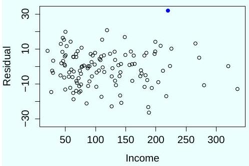
(c) Because the flies were randomly assigned to the five groups, the distribution of thorax lengths in the five groups are essentially equal. What disadvantage would the investigators have incurred by ignoring the thorax length in their analysis (i.e., had they done a one-way ANOVA instead)?
(d) The residual-fitted plot is shown in the left panel of Figure 1 overleaf. Is it possible to determine if the regular residuals or the studentized residuals have been used to construct this plot? Explain.
(e) The Box-Cox procedure was used to determine a good transformation for this data. The plot of the log-likelihood for is shown in the right panel of Figure 1 . What transformation should be used to improve the fit and yet retain some interpretability?
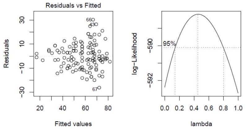
Figure 1: Residual-Fitted plot on the left and Box-Cox plot on the right
Paper 3, Section I, 5K
Consider the linear model
for , where the are independent and identically distributed with distribution. What does it mean for the pair and to be orthogonal? What does it mean for all the three parameters and to be mutually orthogonal? Give necessary and sufficient conditions on so that and are mutually orthogonal. If are mutually orthogonal, find the joint distribution of the corresponding maximum likelihood estimators and .
Paper 4, Section I, K
Define the concepts of an exponential dispersion family and the corresponding variance function. Show that the family of Poisson distributions with parameter is an exponential dispersion family. Find the corresponding variance function and deduce from it expressions for and when . What is the canonical link function in this case?
Paper 4, Section II, K
Let be jointly independent and identically distributed with and conditional on .
(a) Write down the likelihood of the data , and find the maximum likelihood estimate of . [You may use properties of conditional probability/expectation without providing a proof.]
(b) Find the Fisher information for a single observation, .
(c) Determine the limiting distribution of . [You may use the result on the asymptotic distribution of maximum likelihood estimators, without providing a proof.]
(d) Give an asymptotic confidence interval for with coverage using your answers to (b) and (c).
(e) Define the observed Fisher information. Compare the confidence interval in part (d) with an asymptotic confidence interval with coverage based on the observed Fisher information.
(f) Determine the exact distribution of and find the true coverage probability for the interval in part (e). [Hint. Condition on and use the following property of conditional expectation: for random vectors, any suitable function , and ,
Paper 1, Section I, J
Let be independent identically distributed random variables with model function , and denote by and expectation and variance under , respectively. Define . Prove that . Show moreover that if is any unbiased estimator of , then its variance satisfies . [You may use the Cauchy-Schwarz inequality without proof, and you may interchange differentiation and integration without justification if necessary.]
Paper 1, Section II, J
The data consist of the record times in 1984 for 35 Scottish hill races. The columns list the record time in minutes, the distance in miles, and the total height gained during the route. The data are displayed in as follows (abbreviated):
Consider a simple linear regression of time on dist and climb. Write down this model mathematically, and explain any assumptions that you make. How would you instruct to fit this model and assign it to a variable hills. ?
First, we test the hypothesis of no linear relationship to the variables dist and climb against the full model. provides the following ANOVA summary:

Using the information in this table, explain carefully how you would test this hypothesis. What do you conclude?
The command
summary (hills. Im1)
provides the following (slightly abbreviated) summary:

Carefully explain the information that appears in each column of the table. What are your conclusions? In particular, how would you test for the significance of the variable climb in this model?
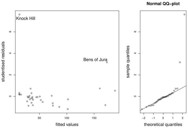
Figure 1: Hills data: diagnostic plots
Finally, we perform model diagnostics on the full model, by looking at studentised residuals versus fitted values, and the normal QQ-plot. The plots are displayed in Figure Comment on possible sources of model misspecification. Is it possible that the problem lies with the data? If so, what do you suggest?
Paper 2, Section I, J
Let be a probability density function, with cumulant generating function . Define what it means for a random variable to have a model function of exponential dispersion family form, generated by . Compute the cumulant generating function of and deduce expressions for the mean and variance of that depend only on first and second derivatives of .
Paper 3, Section I, J
Define a generalised linear model for a sample of independent random variables. Define further the concept of the link function. Define the binomial regression model with logistic and probit link functions. Which of these is the canonical link function?
Paper 4, Section I, J
The numbers of ear infections observed among beach and non-beach (mostly pool) swimmers were recorded, along with explanatory variables: frequency, location, age, and sex. The data are aggregated by group, with a total of 24 groups defined by the explanatory variables.
The data look like this:
Let denote the expected number of ear infections of a person in group . Explain why it is reasonable to model count as Poisson with mean .
We fit the following Poisson model:
where is an offset, i.e. an explanatory variable with known coefficient produces the following (abbreviated) summary for the main effects model:

Why are expressions freq , locB, age , and sexF not listed?
Suppose that we plan to observe a group of 20 female, non-frequent, beach swimmers, aged 20-24. Give an expression (using the coefficient estimates from the model fitted above) for the expected number of ear infections in this group.
Now, suppose that we allow for interaction between variables age and sex. Give the command for fitting this model. We test for the effect of this interaction by producing the following (abbreviated) ANOVA table:

Briefly explain what test is performed, and what you would conclude from it. Does either of these models fit the data well?
Paper 4, Section II, J
Consider the general linear model , where the matrix has full rank , and where has a multivariate normal distribution with mean zero and covariance matrix . Write down the likelihood function for and derive the maximum likelihood estimators of . Find the distribution of . Show further that and are independent.
Paper 1, Section I, J
Consider a binomial generalised linear model for data modelled as realisations of independent and logit for some known constants , and unknown scalar parameter . Find the log-likelihood for , and the likelihood equation that must be solved to find the maximum likelihood estimator of . Compute the second derivative of the log-likelihood for , and explain the algorithm you would use to find .
Paper 1, Section II, J
Consider a generalised linear model with parameter partitioned as , where has components and has components, and consider testing against . Define carefully the deviance, and use it to construct a test for .
[You may use Wilks' theorem to justify this test, and you may also assume that the dispersion parameter is known.]
Now consider the generalised linear model with Poisson responses and the canonical link function with linear predictor given by , where for every . Derive the deviance for this model, and argue that it may be approximated by Pearson's statistic.
Paper 2, Section I, J
Suppose you have a parametric model consisting of probability mass functions . Given a sample from , define the maximum likelihood estimator for and, assuming standard regularity conditions hold, state the asymptotic distribution of .
Compute the Fisher information of a single observation in the case where is the probability mass function of a Poisson random variable with parameter . If are independent and identically distributed random variables having a Poisson distribution with parameter , show that and are unbiased estimators for . Without calculating the variance of , show that there is no reason to prefer over .
[You may use the fact that the asymptotic variance of is a lower bound for the variance of any unbiased estimator.]
Paper 3, Section I, J
Consider the linear model , where is a random vector, , and where the nonrandom matrix is known and has full column rank . Derive the maximum likelihood estimator of . Without using Cochran's theorem, show carefully that is biased. Suggest another estimator for that is unbiased.
Paper 4, Section I, J
Below is a simplified 1993 dataset of US cars. The columns list index, make, model, price (in , miles per gallon, number of passengers, length and width in inches, and weight (in pounds). The data are displayed in as follows (abbreviated):
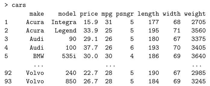
It is reasonable to assume that prices for different makes of car are independent. We model the logarithm of the price as a linear combination of the other quantitative properties of the cars and an error term. Write down this model mathematically. How would you instruct to fit this model and assign it to a variable "fit"?
provides the following (slightly abbreviated) summary:

Briefly explain the information that is being provided in each column of the table. What are your conclusions and how would you try to improve the model?
Paper 4, Section II, J
Every day, Barney the darts player comes to our laboratory. We record his facial expression, which can be either "mad", "weird" or "relaxed", as well as how many units of beer he has drunk that day. Each day he tries a hundred times to hit the bull's-eye, and we write down how often he succeeds. The data look like this:
\begin{tabular}{rrrr} \multicolumn{1}{l}{} & & & \ Day & Beer & Expression & BullsEye \ 1 & 3 & Mad & 30 \ 2 & 3 & Mad & 32 \ & & & \ 60 & 2 & Mad & 37 \ 61 & 4 & Weird & 30 \ & & & \ 110 & 4 & Weird & 28 \ 111 & 2 & Relaxed & 35 \ & & & \ 150 & 3 & Relaxed & 31 \end{tabular}
Write down a reasonable model for , where and where is the number of times Barney has hit bull's-eye on the th day. Explain briefly why we may wish initially to include interactions between the variables. Write the code to fit your model.
The scientist of the above story fitted her own generalized linear model, and subsequently obtained the following summary (abbreviated):

Why are ExpressionMad and Beer:ExpressionMad not listed? Suppose on a particular day, Barney's facial expression is weird, and he drank three units of beer. Give the linear predictor in the scientist's model for this day.
Based on the summary, how could you improve your model? How could one fit this new model in (without modifying the data file)?
Paper 1, Section I, I
Consider a binomial generalised linear model for data , modelled as realisations of independent and , i.e. , for some known constants , and an unknown parameter . Find the log-likelihood for , and the likelihood equations that must be solved to find the maximum likelihood estimator of .
Compute the first and second derivatives of the log-likelihood for , and explain the algorithm you would use to find .
Paper 1, Section II, I
A three-year study was conducted on the survival status of patients suffering from cancer. The age of the patients at the start of the study was recorded, as well as whether or not the initial tumour was malignant. The data are tabulated in as follows:
Describe the model that is being fitted by the following commands:
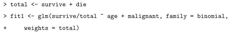
Explain the (slightly abbreviated) output from the code below, describing how the hypothesis tests are performed and your conclusions based on their results.

Based on the summary above, motivate and describe the following alternative model:

Based on the output of the code that follows, which of the two models do you prefer? Why?
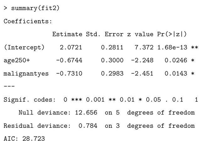
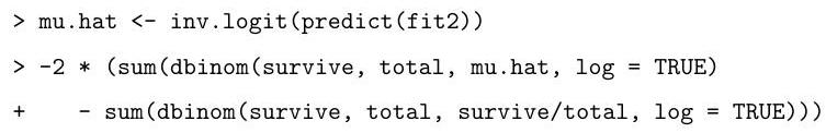
What is the final value obtained by the following commands?
Paper 2, Section I, I
What is meant by an exponential dispersion family? Show that the family of Poisson distributions with parameter is an exponential dispersion family by explicitly identifying the terms in the definition.
Find the corresponding variance function and deduce directly from your calculations expressions for and when .
What is the canonical link function in this case?
Paper 3, Section , I
Consider the linear model , where and is an matrix of full rank . Suppose that the parameter is partitioned into sets as follows: . What does it mean for a pair of sets , to be orthogonal? What does it mean for all sets to be mutually orthogonal?
In the model
where are independent and identically distributed, find necessary and sufficient conditions on for and to be mutually orthogonal.
If and are mutually orthogonal, what consequence does this have for the joint distribution of the corresponding maximum likelihood estimators and ?
Paper 4, Section I,
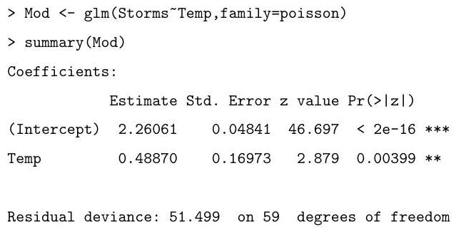
Sulphur dioxide is one of the major air pollutants. A dataset by Sokal and Rohlf (1981) was collected on 41 US cities/regions in 1969-1971. The annual measurements obtained for each region include (average) sulphur dioxide content, temperature, number of manufacturing enterprises employing more than 20 workers, population size in thousands, wind speed, precipitation, and the number of days with precipitation. The data are displayed in as follows (abbreviated):

Describe the model being fitted by the following commands.
fit temp manuf pop wind precip days
Explain the (slightly abbreviated) output below, describing in particular how the hypothesis tests are performed and your conclusions based on their results:
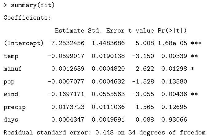
Based on the summary above, suggest an alternative model.
Finally, what is the value obtained by the following command?
Paper 4, Section II, I
Consider the linear model , where and is an matrix of full rank . Find the form of the maximum likelihood estimator of , and derive its distribution assuming that is known.
Assuming the prior find the joint posterior of up to a normalising constant. Derive the posterior conditional distribution .
Comment on the distribution of found above and the posterior conditional . Comment further on the predictive distribution of at input under both the maximum likelihood and Bayesian approaches.
Suppose that we want to estimate the angles and (in radians, say) of the triangle , based on a single independent measurement of the angle at each corner. Suppose that the error in measuring each angle is normally distributed with mean zero and variance . Thus, we model our measurements as the observed values of random variables
where are independent, each with distribution . Find the maximum likelihood estimate of based on these measurements.
Can the assumption that be criticized? Why or why not?
1.I.5J
Consider the following Binomial generalized linear model for data , with logit link function. The data are regarded as observed values of independent random variables , where
where is an unknown -dimensional parameter, and where are known dimensional explanatory variables. Write down the likelihood function for under this model.
Show that the maximum likelihood estimate satisfies an equation of the form , where is the matrix with rows , and where , with a function of and , which you should specify.
Define the deviance and find an explicit expression for in terms of and in the case of the model above.
1.II.13J
Consider performing a two-way analysis of variance (ANOVA) on the following data:
Explain and interpret the R commands and (slightly abbreviated) output below. In particular, you should describe the model being fitted, and comment on the hypothesis tests which are performed under the summary and anova commands.
[1]
as.vector
, length
, length
Coefficients:
Estimate Std. Error t value
(Intercept)
b2
b3
The following code fits a similar model. Briefly explain the difference between this model and the one above. Based on the output of the anova call below, say whether you prefer this model over the one above, and explain your preference.

Finally, explain what is being calculated in the code below and give the value that would be obtained by the final line of code.
3.I.5J
Consider the linear model . Here, is an -dimensional vector of observations, is a known matrix, is an unknown -dimensional parameter, and , with unknown. Assume that has full rank and that . Suppose that we are interested in checking the assumption . Let , where is the maximum likelihood estimate of . Write in terms of an expression for the projection matrix which appears in the maximum likelihood equation .
Find the distribution of , and show that, in general, the components of are not independent.
A standard procedure used to check our assumption on is to check whether the studentized fitted residuals
look like a random sample from an distribution. Here,
Say, briefly, how you might do this in R.
This procedure appears to ignore the dependence between the components of noted above. What feature of the given set-up makes this reasonable?
4.I
A long-term agricultural experiment had grassland plots, each , differing in biomass, soil pH, and species richness (the count of species in the whole plot). While it was well-known that species richness declines with increasing biomass, it was not known how this relationship depends on soil pH. In the experiment, there were 30 plots of "low pH", 30 of "medium pH" and 30 of "high pH". Three lines of the data are reproduced here as an aid.
Briefly explain the commands below. That is, explain the models being fitted.
Let and denote the hypotheses represented by the three models and fits. Based on the output of the code below, what hypotheses are being tested, and which of the models seems to give the best fit to the data? Why?

Finally, what is the value obtained by the following command?

4.II.13J
Consider the following generalized linear model for responses as a function of explanatory variables , where for . The responses are modelled as observed values of independent random variables , with
Here, is a given link function, and are unknown parameters, and the are treated as known.
[Hint: recall that we write to mean that has density function of the form
for given functions a and
[ You may use without proof the facts that, for such a random variable ,
Show that the score vector and Fisher information matrix have entries:
and
How do these expressions simplify when the canonical link is used?
Explain briefly how these two expressions can be used to obtain the maximum likelihood estimate for .
1.I.5I
According to the Independent newspaper (London, 8 March 1994) the Metropolitan Police in London reported 30475 people as missing in the year ending March 1993. For those aged 18 or less, 96 of 10527 missing males and 146 of 11363 missing females were still missing a year later. For those aged 19 and above, the values were 157 of 5065 males and 159 of 3520 females. This data is summarised in the table below.
\begin{array}{rrrrr} & \multicolumn{3}{r}{\text { age }} \\ 1 & \text { Kender } & \text { M } & 96 & 10527 \\ 2 & \text { Kid } & \text { F } & 146 & 11363 \\ 3 & \text { Adult } & \text { M } & 157 & 5065 \\ 4 & \text { Adult } & \text { F } & 159 & 3520 \end{array}
Explain and interpret the commands and (slightly abbreviated) output below. You should describe the model being fitted, explain how the standard errors are calculated, and comment on the hypothesis tests being described in the summary. In particular, what is the worst of the four categories for the probability of remaining missing a year later?
For a person who was missing in the year ending in March 1993, find a formula, as a function of age and gender, for the estimated expected probability that they are still missing a year later.
1.II.13I
This problem deals with data collected as the number of each of two different strains of Ceriodaphnia organisms are counted in a controlled environment in which reproduction is occurring among the organisms. The experimenter places into the containers a varying concentration of a particular component of jet fuel that impairs reproduction. Hence it is anticipated that as the concentration of jet fuel grows, the mean number of organisms should decrease.
The table below gives a subset of the data. The full dataset has rows. The first column provides the number of organisms, the second the concentration of jet fuel (in grams per litre) and the third specifies the strain of the organism.
Explain and interpret the commands and (slightly abbreviated) output below. In particular, you should describe the model being fitted, explain how the standard errors are calculated, and comment on the hypothesis tests being described in the summary.
The following code fits two very similar models. Briefly explain the difference between these models and the one above. Motivate the fitting of these models in light of
Part II 2007 the summary from the fit of the one above.
Denote by the three hypotheses being fitted in sequence above.
Explain the hypothesis tests, including an approximate test of the fit of , that can be performed using the output from the following code. Use these numbers to comment on the most appropriate model for the data.
, fit2$dev, fit3$dev)
[1]
[1]
2.I.5I
Consider the linear regression setting where the responses are assumed independent with means . Here is a vector of known explanatory variables and is a vector of unknown regression coefficients.
Show that if the response distribution is Laplace, i.e.,
then the maximum likelihood estimate of is obtained by minimising
Obtain the maximum likelihood estimate for in terms of .
Briefly comment on why the Laplace distribution cannot be written in exponential dispersion family form.
3.I.5I
Consider two possible experiments giving rise to observed data where
- The data are realizations of independent Poisson random variables, i.e.,
where , with an unknown (possibly vector) parameter. Write for the maximum likelihood estimator (m.l.e.) of and for the th fitted value under this model.
- The data are components of a realization of a multinomial random 'vector'
where the are non-negative integers with
Write for the m.l.e. of and for the th fitted value under this model.
Show that, if
then and for all . Explain the relevance of this result in the context of fitting multinomial models within a generalized linear model framework.
4.I.5I
Consider the normal linear model in vector notation, where
i.i.d. ,
where is known and is of full rank . Give expressions for maximum likelihood estimators and of and respectively, and state their joint distribution.
Suppose that there is a new pair , independent of , satisfying the relationship
We suppose that is known, and estimate by . State the distribution of
Find the form of a -level prediction interval for .
4.II.13I
Let have a Gamma distribution with density
Show that the Gamma distribution is of exponential dispersion family form. Deduce directly the corresponding expressions for and in terms of and . What is the canonical link function?
Let . Consider a generalised linear model (g.l.m.) for responses with random component defined by the Gamma distribution with canonical link , so that , where is the vector of unknown regression coefficients and is the vector of known values of the explanatory variables for the th observation, .
Obtain expressions for the score function and Fisher information matrix and explain how these can be used in order to approximate , the maximum likelihood estimator (m.l.e.) of .
[Use the canonical link function and assume that the dispersion parameter is known.]
Finally, obtain an expression for the deviance for a comparison of the full (saturated) model to the g.l.m. with canonical link using the m.l.e. (or estimated mean .
1.I.5I
Assume that observations satisfy the linear model
where is an matrix of known constants of full , where is unknown and . Write down a -level confidence set for .
Define Cook's distance for the observation , where is the th row of . Give its interpretation in terms of confidence sets for .
In the above model with and , you observe that one observation has Cook's distance 1.3. Would you be concerned about the influence of this observation?
[You may find some of the following facts useful:
(i) If , then and .
(ii) If , then and .
(iii) If , then and . ]
1.II.13I
The table below gives a year-by-year summary of the career batting record of the baseball player Babe Ruth. The first column gives his age at the start of each season and the second gives the number of 'At Bats' (AB) he had during the season. For each At Bat, it is recorded whether or not he scored a 'Hit'. The third column gives the total number of Hits he scored in the season, and the final column gives his 'Average' for the season, defined as the number of Hits divided by the number of At Bats.
Explain and interpret the commands below. In particular, you should explain the model that is being fitted, the approximation leading to the given standard errors and the test that is being performed in the last line of output.

Assuming that any required packages are loaded, draw a careful sketch of the graph that you would expect to see on entering the following lines of code:
2.I.5I
Let be independent Poisson random variables with means , for , where , for some known constants and an unknown parameter . Find the log-likelihood for .
By first computing the first and second derivatives of the log-likelihood for , explain the algorithm you would use to find the maximum likelihood estimator, .
3.I.5I
Consider a generalized linear model for independent observations , with for . What is a linear predictor? What is meant by the link function? If has model function (or density) of the form
for , where is a known positive function, define the canonical link function.
Now suppose that are independent with for . Derive the canonical link function.
4.I.5I
The table below summarises the yearly numbers of named storms in the Atlantic basin over the period 1944-2004, and also gives an index of average July ocean temperature in the northern hemisphere over the same period. To save space, only the data for the first four and last four years are shown.
Explain and interpret the commands and (slightly abbreviated) output below.
In 2005 , the ocean temperature index was 0.743. Explain how you would predict the number of named storms for that year.
4.II.13I
Consider a linear model for given by
where is a known matrix of full rank , where is an unknown vector and . Derive an expression for the maximum likelihood estimator of , and write down its distribution.
Find also the maximum likelihood estimator of , and derive its distribution.
[You may use Cochran's theorem, provided that it is stated carefully. You may also assume that the matrix has rank , and that has rank .]
1.I.5I
Suppose that are independent random variables, and that has probability density function
Assume that and that there is a known link function such that
where are known -dimensional vectors and is an unknown -dimensional parameter. Show that and that, if is the log-likelihood function from the observations , then
where is to be defined.
1.II.13I
The Independent, June 1999 , under the headline 'Tourists get hidden costs warnings' gave the following table of prices in pounds, called 'How the resorts compared'.
Here the column headings are, respectively: Three-course meal, Bottle of Beer, Suntan Lotion, Taxi (5km), Film (24 exp), Car Hire (per week). Interpret the commands, and explain how to interpret the corresponding (slightly abbreviated) output given below. Your solution should include a careful statement of the underlying statistical model, but you may quote without proof any distributional results required.
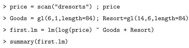
Residual standard error: on 65 degrees of freedom
Multiple R-Squared:
2.I.5I
You see below three commands, and the corresponding output (which is slightly abbreviated). Explain the effects of the commands. How is the deviance defined, and why do we have d.f. in this case? Interpret the numerical values found in the output.
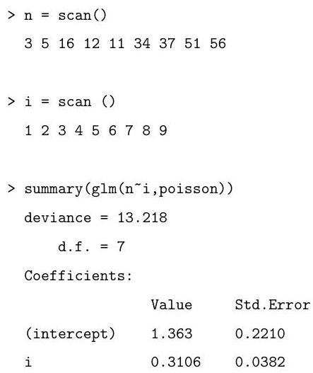
3.I.5I
Consider the model , where is an -dimensional observation vector, is an matrix of rank is an -dimensional vector with components , and are independently and normally distributed, each with mean 0 and variance
(a) Let be the least-squares estimator of . Show that
and find the distribution of .
(b) Define . Show that has distribution , where is a matrix that you should define.
[You may quote without proof any results you require about the multivariate normal distribution.]
4.I.5I
You see below five commands, and the corresponding output (which is slightly abbreviated). Without giving any mathematical proofs, explain the purpose of these commands, and interpret the output.

Residual deviance: on 2 degrees of freedom
Number of Fisher Scoring iterations: 4
4.II.13I
(i) Suppose that are independent random variables, and that has probability density function
where
and are given -dimensional vectors, and is known.
Show that and that .
(ii) Find the equation for , the maximum likelihood estimator of , and suggest an iterative scheme for its solution.
(iii) If , and , find the large-sample distribution of . Write your answer in terms of and , where are defined by