Computational Statistics And Statistical Modelling
Computational Statistics And Statistical Modelling
Jump to year
A1.13
(i) Assume that the -dimensional vector may be written as , where is a given matrix of is an unknown vector, and
Let . Find , the least-squares estimator of , and state without proof the joint distribution of and .
(ii) Now suppose that we have observations and consider the model
where are fixed parameters with , and may be assumed independent normal variables, with , where is unknown.
(a) Find , the least-squares estimators of .
(b) Find the least-squares estimators of under the hypothesis for all .
(c) Quoting any general theorems required, explain carefully how to test , assuming is true.
(d) What would be the effect of fitting the model , where now are all fixed unknown parameters, and has the distribution given above?
A2.12
(i) Suppose we have independent observations , and we assume that for is Poisson with mean , and , where are given covariate vectors each of dimension , where is an unknown vector of dimension , and . Assuming that span , find the equation for , the maximum likelihood estimator of , and write down the large-sample distribution of .
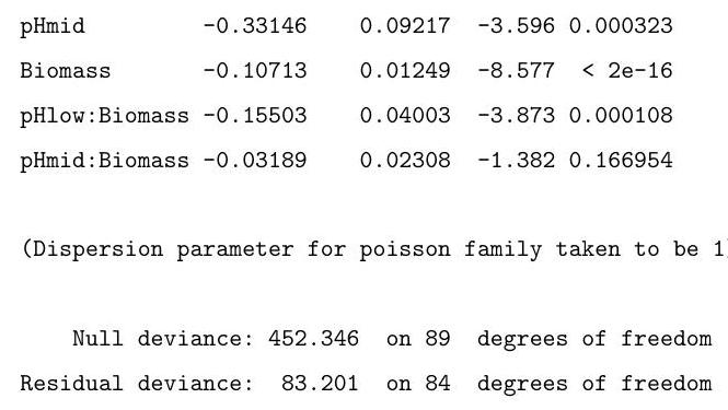
(ii) A long-term agricultural experiment had 90 grassland plots, each , differing in biomass, soil pH, and species richness (the count of species in the whole plot). While it was well-known that species richness declines with increasing biomass, it was not known how this relationship depends on soil pH, which for the given study has possible values "low", "medium" or "high", each taken 30 times. Explain the commands input, and interpret the resulting output in the (slightly edited) output below, in which "species" represents the species count.
(The first and last 2 lines of the data are reproduced here as an aid. You may assume that the factor pH has been correctly set up.)


A4.14
Suppose that are independent observations, with having probability density function of the following form
where and . You should assume that is a known function, and are unknown parameters, with , and also are given linearly independent covariate vectors. Show that
where is the log-likelihood and .
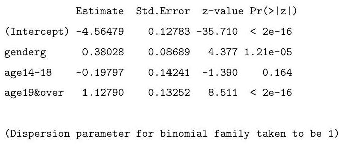
Discuss carefully the (slightly edited) output given below, and briefly suggest another possible method of analysis using the function ( ).
1:
7:
Read 6 items
1: 327172565065248688773520
Read 6 items
gender <-
1: b b b g g g
Read 6 items
age <-
1: 13&under 14-18 19&over
4: 13&under 14-18 19&over
7 :
Read 6 items
gender <- factor (gender) ; age <- factor (age)
gender age, binomial, weights
Coefficients:

Null deviance: on 5 degrees of freedom
Residual deviance: on 2 degrees of freedom
Number of Fisher Scoring iterations: 3
A1.13
(i) Suppose , are independent binomial observations, with , , where are known, and we wish to fit the model
where are given covariates, each of dimension . Let be the maximum likelihood estimators of . Derive equations for and state without proof the form of the approximate distribution of .
(ii) In 1975 , data were collected on the 3-year survival status of patients suffering from a type of cancer, yielding the following table
\begin{tabular}{ccrr} & & \multicolumn{2}{c}{ survive? } \ age in years & malignant & yes & no \ under 50 & no & 77 & 10 \ under 50 & yes & 51 & 13 \ & no & 51 & 11 \ & yes & 38 & 20 \ & no & 7 & 3 \ & yes & 6 & 3 \end{tabular}
Here the second column represents whether the initial tumour was not malignant or was malignant.
Let be the number surviving, for age group and malignancy status , for and , and let be the corresponding total number. Thus , . Assume . The results from fitting the model
with give , and deviance . What do you conclude?
Why do we take in the model?
What "residuals" should you compute, and to which distribution would you refer them?
A2.12
(i) Suppose are independent Poisson variables, and
where are two unknown parameters, and are given covariates, each of dimension 1. Find equations for , the maximum likelihood estimators of , and show how an estimate of may be derived, quoting any standard theorems you may need.
(ii) By 31 December 2001, the number of new vCJD patients, classified by reported calendar year of onset, were
for the years
Discuss carefully the (slightly edited) output for these data given below, quoting any standard theorems you may need.
year
year
[1] 1994199519961997199819992000
tot
[1]
first.glm - glm(tot year, family = poisson)
(first.glm)
Call:
glm(formula tot year, family poisson
Coefficients
Estimate Std. Error z value
(Intercept)
year
(Dispersion parameter for poisson family taken to be 1)
Null deviance: on 6 degrees of freedom
Residual deviance: on 5 degrees of freedom
Number of Fisher Scoring iterations: 3
Part II 2003
A4.14
The nave height , and the nave length for 16 Gothic-style cathedrals and 9 Romanesque-style cathedrals, all in England, have been recorded, and the corresponding output (slightly edited) is given below.

You may assume that are in suitable units, and that "style" has been set up as a factor with levels 1,2 corresponding to Gothic, Romanesque respectively.
(a) Explain carefully, with suitable graph(s) if necessary, the results of this analysis.
(b) Using the general model (in the conventional notation) explain carefully the theory needed for (a).
[Standard theorems need not be proved.]
A1.13
(i) Suppose are independent Poisson variables, and
where are unknown parameters, and are given covariates, each of dimension . Obtain the maximum-likelihood equations for , and explain briefly how you would check the validity of this model.
(ii) The data below show , which are the monthly accident counts on a major US highway for each of the 12 months of 1970 , then for each of the 12 months of 1971 , and finally for the first 9 months of 1972 . The data-set is followed by the (slightly edited) output. You may assume that the factors 'Year' and 'month' have been set up in the appropriate fashion. Give a careful interpretation of this output, and explain (a) how you would derive the corresponding standardised residuals, and (b) how you would predict the number of accidents in October 1972 .
first.glm Year month, poisson summary(first.glm
Call:
formula Year month, family poisson
\begin{tabular}{lrlll} Coefficients: & & & & \ (Intercept) & Estimate & Std. Error & \multicolumn{1}{l}{ z value } & \ Year1971 & & & & \ Year1972 & & & & \ month2 & & & & \ month3 & & & & \ month4 & & & & \ month5 & & & & \ month6 & & & & \ month7 & & & & \ month8 & & & & \ month9 & & & & \ month10 & & & & \ month11 & & & & \ month12 & & & & \end{tabular}
Signif. codes: 0 (, (, (, '.
(Dispersion parameter for poisson family taken to be 1 )
Number of Fisher Scoring iterations: 3
A2.12
(i) Suppose that the random variable has density function of the form
where . Show that has expectation and variance .
(ii) Suppose now that are independent negative exponential variables, with having density function for . Suppose further that for , where is a known 'link' function, and are given covariate vectors, each of dimension . Discuss carefully the problem of finding , the maximum-likelihood estimator of , firstly for the case , and secondly for the case ; in both cases you should state the large-sample distribution of .
[Any standard theorems used need not be proved.]
A4.14
Assume that the -dimensional observation vector may be written as , where is a given matrix of rank is an unknown vector, with , and
where is unknown. Find , the least-squares estimator of , and describe (without proof) how you would test
for a given .
Indicate briefly two plots that you could use as a check of the assumption .
Continued opposite Sulphur dioxide is one of the major air pollutants. A data-set presented by Sokal and Rohlf (1981) was collected on 41 US cities in 1969-71, corresponding to the following variables:
sulphur dioxide content of air in micrograms per cubic metre
average annual temperature in degrees Fahrenheit
= number of manufacturing enterprises employing 20 or more workers
population size (1970 census) in thousands
average annual wind speed in miles per hour
average annual precipitation in inches
average annual of days with precipitation per year
Interpret the output that follows below, quoting any standard theorems that you need to use.
Residuals :
Signif. codes: 0 ', ', ', ':
Residual standard error: on 34 degrees of freedom
Multiple R-Squared:
F-statistic: on 6 and 34 degrees of freedom, p-value:
A1.13
(i) Assume that the -dimensional observation vector may be written as
where is a given matrix of is an unknown vector, and
Let . Find , the least-squares estimator of , and show that
where is a matrix that you should define.
(ii) Show that . Show further for the special case of
where , that
here, is a vector of which every element is one, and , are constants that you should derive.
Hence show that, if is the vector of fitted values, then
A2.12
(i) Suppose that are independent random variables, and that has probability density function
Assume that , and that , where is a known 'link' function, are known covariates, and is an unknown vector. Show that
and hence
(ii) The table below shows the number of train miles (in millions) and the number of collisions involving British Rail passenger trains between 1970 and 1984 . Give a detailed interpretation of the output that is shown under this table:
Call:
glm(formula collisions year miles , family poisson)
Coefficients:
(Dispersion parameter for poisson family taken to be 1)
Null deviance: on 13 degrees of freedom
Residual deviance: on 11 degrees of freedom
Number of Fisher Scoring iterations: 4
Part II
A4.14
(i) Assume that independent observations are such that
where are given covariates. Discuss carefully how to estimate , and how to test that the model fits.
(ii) Carmichael et al. (1989) collected data on the numbers of 5 -year old children with "dmft", i.e. with 5 or more decayed, missing or filled teeth, classified by social class, and by whether or not their tap water was fluoridated or non-fluoridated. The numbers of such children with dmft, and the total numbers, are given in the table below:
\begin{tabular}{l|ll} Social Class & Fluoridated & Non-fluoridated \ \hline I & & \ II & & \ III & & \ Unclassified & & \end{tabular}
A (slightly edited) version of the output is given below. Explain carefully what model is being fitted, whether it does actually fit, and what the parameter estimates and Std. Errors are telling you. (You may assume that the factors SClass (social class) and Fl (with/without) have been correctly set up.)


Here 'Yes' is the vector of numbers with dmft, taking values , 'Total' is the vector of Total in each category, taking values , and SClass, Fl are the factors corresponding to Social class and Fluoride status, defined in the obvious way.