A scientist is studying the effects of a drug on the weight of mice. Forty mice are divided into two groups, control and treatment. The mice in the treatment group are given the drug, and those in the control group are given water instead. The mice are kept in 8 different cages. The weight of each mouse is monitored for 10 days, and the results of the experiment are recorded in the data frame Weight.data. Consider the following $R$ code and its output.

head (Weight.data)

Time Group Cage Mouse Weight

11 Control 1 1 $24.77578$

$2 \quad 2$ Control 1 1 $24.68766$

$3 \quad 3$ Control $1 \quad 124.79008$

44 Control $1 \quad 124.77005$

$5 \quad 5$ Control 1 1 $24.65092$

$6 \quad 6$ Control $1 \quad 124.38436$

$>\bmod 1=\operatorname{lm}$ (Weight $\sim$ Time*Group $+$ Cage, data=Weight. data)

$>\operatorname{summary}(\bmod 1)$

Call:

$\operatorname{lm}$ (formula $=$ Weight $~$Time $*$ Group $+$ Cage, data $=$ Weight. data)

Residuals:

Min $1 Q$ Median $3 Q$ Max

$-1.36903-0.33527-0.01719 \quad 0.38807 \quad 1.24368$

Coefficients:

Estimate Std. Error t value $\operatorname{Pr}(>|t|)$

$\begin{array}{lllll}\text { Time } & -0.006023 & 0.012616 & -0.477 & 0.63334\end{array}$

GroupTreatment $\quad 0.321837 \quad 0.121993 \quad 2.638 \quad 0.00867 *$

Cage2 $\quad-0.400228 \quad 0.095875-4.1743 .68 \mathrm{e}-05 * * *$

$\begin{array}{lllll}\text { Cage3 } & 0.286941 & 0.102494 & 2.800 & 0.00537 *\end{array}$

$\begin{array}{lllll}\text { Cage4 } & 0.007535 & 0.095875 & 0.079 & 0.93740\end{array}$

$\begin{array}{rrrrr}\text { Cage6 } & 0.124767 & 0.125530 & 0.994 & 0.32087\end{array}$

$\begin{array}{lllll}\text { Cage8 } & -0.295168 & 0.125530 & -2.351 & 0.01920 * \\ \text { Time:GroupTreatment } & -0.173515 & 0.017842 & -9.725 & <2 e-16 * * *\end{array}$

Time: GroupTreatment $-0.173515 \quad 0.017842-9.725<2 \mathrm{e}-16 * * *$

Signif. codes: 0 '' $0.001$ '' $0.01$ '' $0.05$ '., $0.1$ ', 1

Residual standard error: $0.5125$ on 391 degrees of freedom

Multiple R-squared: $0.5591$, Adjusted R-squared: $0.55$

F-statistic: $61.97$ on 8 and 391 DF, p-value: $<2.2 \mathrm{e}-16$

Which parameters describe the rate of weight loss with time in each group? According to the $\mathrm{R}$ output, is there a statistically significant weight loss with time in the control group?

Three diagnostic plots were generated using the following $R$ code.

Weight.data$Time[mouse1]

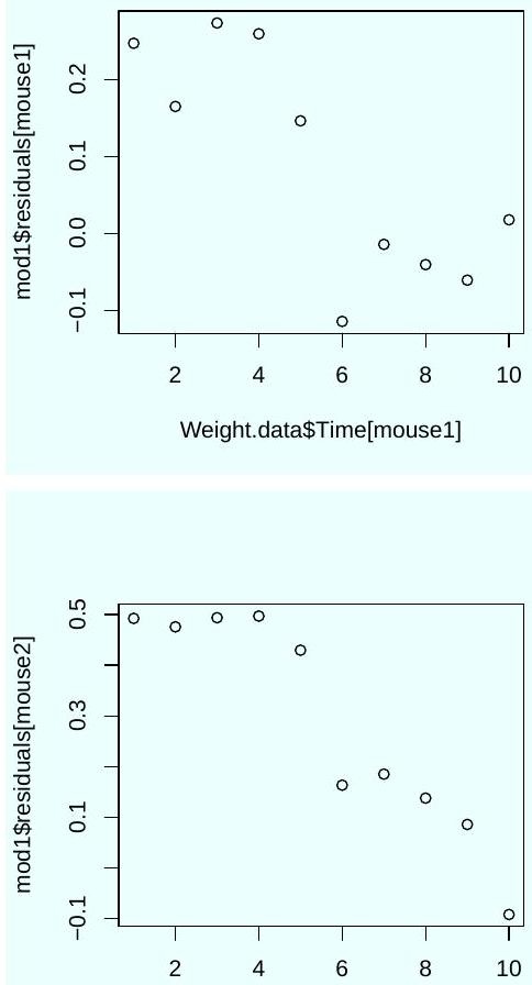
Weight.data$Time[mouse2]

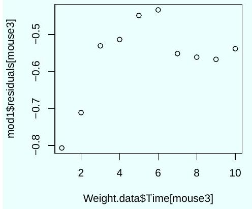
Based on these plots, should you trust the significance tests shown in the output of the command summary (mod1)? Explain.